Plotting Trees and Heatmaps
DLP data is commonly vizualized as a heatmap of copy number states across the genome.
Next to this heatmap, we often want to add:
- phylogenetic trees of the cellular relationships
- annotations of sample, experiments
- clonal identities both as labels and colors on the tree
The package Signals has great functions to do this (and lots of other useful functions for DLP and single cell analyses).
Alternatively, in this package there is
dlptools::plot_state_hm(), which does similar things to the
Signals package, but with some more conveniences.
dlptools::plot_state_hm() is meant to be a one stop shop
for heatmap plotting of many variable types and options (click that link
for all of the options).
The main constraint is to have a column called cell_id
that contains the cell labels.
We’ll work from some example data to show some examples (it’s a trimmed output of signals, but just DLP reads output works fine too):
ex_state_dat <- vroom::vroom("data/ex_state_dat.tsv.gz")

head(ex_state_dat)
#> # A tibble: 6 × 11
#>   cell_id sample_id passage   chr  start    end state   BAF state_AS state_phase
#>   <chr>   <chr>     <chr>   <dbl>  <dbl>  <dbl> <dbl> <dbl> <chr>    <chr>
#> 1 AT2399… AT23998   p1          1 2.00e6 2.5 e6     4 0.179 3|1      A-Gained
#> 2 AT2399… AT23998   p1          1 3.00e6 3.5 e6     4 0.294 3|1      A-Gained
#> 3 AT2399… AT23998   p1          1 4.00e6 4.50e6     4 0.211 3|1      A-Gained
#> 4 AT2399… AT23998   p1          1 4.50e6 5   e6     5 0.299 5        A-Gained
#> 5 AT2399… AT23998   p1          1 5.00e6 5.50e6     5 0.182 5        A-Gained
#> 6 AT2399… AT23998   p1          1 5.50e6 6   e6     5 0.129 5        A-Gained
#> # ℹ 1 more variable: copy <dbl>
basic heatmap
dlptools::plot_state_hm(
  states_df = ex_state_dat,
  state_col = "state",
  # optional, but recommended dump direct to a file with:
  file_name = "imgs/basic_hm.png"
  # recommended for full, large, heatmaps
  # optional for HMMcopy state data, 11 is really 11+, so we can display the
  # legend that way with
  # legend_11plus=TRUE
)
Or with a different column:
dlptools::plot_state_hm(
  states_df = ex_state_dat,
  state_col = "state_phase",
  # optional, but recommended dump direct to a file with:
  file_name = "imgs/basic_phase_hm.png"
  # recommended for full, large, heatmaps
)
Column options include:
- state
- state_phase (A-gained, B-hom, etc)
- A
- B
- BAF
- state_AS
- state_AS_phased (might be too many states to usefully visualize)
- or pretty much any custom column you want to plot that is reasonably similar.
Adding a Tree
ex_tree <- ape::read.tree("data/pkg_tree.newick")

dlptools::plot_state_hm(
  states_df = ex_state_dat,
  state_col = "state",
  phylogeny = ex_tree,
  file_name = "imgs/with_tree_hm.png"
)
Adding Annotation Data
This can come from a separate data frame with annotations per cell ID, or you can point to columns in your state dataframe:
dlptools::plot_state_hm(
  states_df = dplyr::mutate(ex_state_dat, passage = as.factor(passage)),
  state_col = "state",
  file_name = "imgs/annotations_hm.png",
  anno_columns = c("sample_id", "passage"),
  # you could control the colors of your annotations with:
  # anno_colors_list = list(passage=c(`1`='#2872bc', `19`='#d23e3e')),
)
Or with some pre-made annotation dataframe created by cell id:
anno_df <- dplyr::distinct(ex_state_dat, cell_id, sample_id, passage)


dlptools::plot_state_hm(
  states_df = ex_state_dat,
  state_col = "state",
  anno_df = anno_df,
  file_name = "imgs/annotations_2_hm.png"
)
And with either of these, we can add a tree with the
phylogeny arguments.
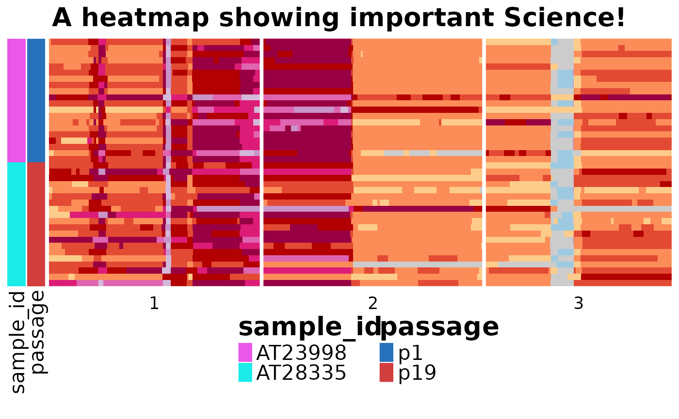
Annotation and Legends
We can also control aspects of the legend and plot title with some options:
dlptools::plot_state_hm(
  states_df = dplyr::mutate(ex_state_dat, passage = as.factor(passage)),
  state_col = "state",
  anno_columns = c("sample_id", "passage"),
  # file_name = "your_heatmap.png" ## still good idea to drop direct to file
  # you could control the colors of your annotations with:
  anno_colors_list = list(passage = c(p1 = "#2872bc", p19 = "#d23e3e")),
  # can turn off the legend for the heatmap values
  show_heatmap_legend = FALSE,
  # can show, or not, the annotation legend
  show_annotation_legend = TRUE,
  # can set a title
  hm_title = "A heatmap showing important Science!",
  # and aspects of the display sizes for titles and labels
  annotation_legend_param = list(
    title_gp = grid::gpar(fontsize = 20, fontface = "bold"),
    labels_gp = grid::gpar(fontsize = 16),
    gp = grid::gpar(fontsize = 5)
  )
)
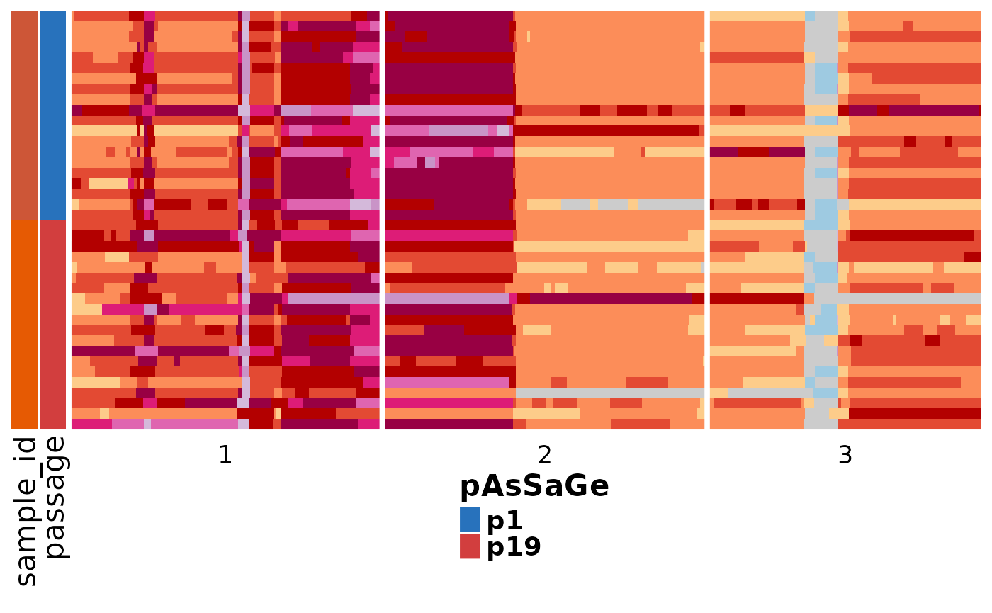
We can also build a fully custom legend…but takes some work, and
you’d probably want a pretty good understanding of
ComplexHeatmap::packLegend:
dlptools::plot_state_hm(
  states_df = dplyr::mutate(ex_state_dat, passage = as.factor(passage)),
  state_col = "state",
  anno_columns = c("sample_id", "passage"),
  # file_name = "your_heatmap.png" ## still good idea to drop direct to file
  # turn off default legends
  show_heatmap_legend = FALSE,
  show_annotation_legend = FALSE,
  anno_colors_list = list(passage = c(p1 = "#2872bc", p19 = "#d23e3e")),
  # and aspects of the display sizes for titles and labels
  custom_legend = ComplexHeatmap::packLegend(
    ComplexHeatmap::Legend(
      title = "pAsSaGe",
      labels = unique(ex_state_dat$passage),
      # would need to match colours above
      legend_gp = grid::gpar(fill = c(p1 = "#2872bc", p19 = "#d23e3e")),
      labels_gp = grid::gpar(fontsize = 14, fontface = "bold"),
      title_gp = grid::gpar(fontsize = 16, fontface = "bold")
    )
  )
)
Clone Information
Clones work similar to annotations, where you can either supply a
data frame with cell_id and clone_id columns,
or just pull the information from the states dataframe:
# fake some clone data
ex_state_dat <- ex_state_dat |>
  dplyr::mutate(
    clone = dplyr::if_else(passage == "p1", "A", "B"),
  )


dlptools::plot_state_hm(
  states_df = ex_state_dat,
  state_col = "state_phase",
  file_name = "imgs/with_clones.png",
  clone_column = "clone",
  # optional, don't have to have annotations, or could pass the dataframe like
  # above
  anno_columns = c("sample_id", "passage"),
  # optional, don't have to have tree
  phylogeny = ex_tree,
  # optional, turns on tree coloring by clone
  color_tree_clones = TRUE,
  # optional, only largest cell group of a clone gets a letter label.
  only_largest_clone_group = TRUE
)
Continous Variables
dlptools::plot_state_hm(
  states_df = ex_state_dat,
  state_col = "copy",
  continuous_hm_colours = TRUE,
  # optional, can specify the colors
  # custom_continuous_colors = c("#000000", "#ffffff", "#5F9EA0")
  # optional, can specify values to fill out low, mid, high end of range
  # basically has the effect of squishing or stretching the color scale
  # custom_continuous_range = c(0, 2, 10)
  file_name = "imgs/continuous.png"
)

# and all of this can be specified with annotations, trees, etc.
# as above.