Various Functions
useful_functions.RmdVarious Functions dlptools
Masking Bad Regions
Masking regions that are bad for DLP, mostly the consequence of low mappability.
# assuming some sort of reads or segments DF with: chr, start, end
ex_reads <- vroom::vroom("data/example_reads.tsv.gz")

ex_reads <- dlptools::mark_mask_regions(ex_reads)

# adds a boolean `mask` column
ex_reads |>
  dplyr::select(cell_id, chr, start, end, mask) |>
  dplyr::slice_head(n = 5)
#> # A tibble: 5 × 5
#>   cell_id                  chr     start     end mask
#>   <chr>                    <chr>   <dbl>   <dbl> <lgl>
#> 1 AT23998-A138956A-R03-C34 1           1  500000 FALSE
#> 2 AT23998-A138956A-R03-C34 1      500001 1000000 FALSE
#> 3 AT23998-A138956A-R03-C34 1     1000001 1500000 FALSE
#> 4 AT23998-A138956A-R03-C34 1     1500001 2000000 FALSE
#> 5 AT23998-A138956A-R03-C34 1     2000001 2500000 FALSE
The default masking file is one constructed by Daniel Lai, and can be viewed at the package source or by loading:
vroom::vroom(system.file("extdata", "blacklist_2023.07.17.txt", package = "dlptools"))
#> # A tibble: 26 × 4
#>    seqnames     start       end    width
#>    <chr>        <dbl>     <dbl>    <dbl>
#>  1 1        120500001 148000000 27500000
#>  2 2         87000001  95500000  8500000
#>  3 3         90500001  93500000  3000000
#>  4 4         49000001  53000000  4000000
#>  5 5         46000001  49500000  3500000
#>  6 6         57000001  62500000  5500000
#>  7 7         55500001  66000000 10500000
#>  8 8         43500001  48000000  4500000
#>  9 9         38500001  71000000 32500000
#> 10 10        38500001  52000000 13500000
#> # ℹ 16 more rows
Marking Centromere Locations
Centromeres are problematic for DLP data, the state calls are often inflated and highly inconsistent between adjacent bins. It’s a messy region that we often want to omit. The default masking file (above) pretty much captures these regions, but sometimes we may want to be more specific.
Alternatively, sometimes we want to specify windows around centromeres to include in filtering too.
The files loaded to mark centromeres come from UCSC cytoband files of hg19 and hg38 releases.
# easiest way is to just explictly mark whether bins are in centromeres
dlptools::mark_bins_overlapping_centromeres(
  reads_df = ex_reads,
  padding = 3e6, # e.g., specifying 3 Mb on each side of centromere
  # default padding is 0
  version = "hg19", # default, don't neeed to specify. Alternative is "hg38"
) |>
  dplyr::count(cell_id, overlaps_centro) |>
  dplyr::slice_head(n = 6)
#> # A tibble: 6 × 3
#>   cell_id                  overlaps_centro     n
#>   <chr>                    <lgl>           <int>
#> 1 AT23998-A138956A-R03-C34 FALSE            5685
#> 2 AT23998-A138956A-R03-C34 TRUE              521
#> 3 AT23998-A138956A-R04-C58 FALSE            5685
#> 4 AT23998-A138956A-R04-C58 TRUE              521
#> 5 AT23998-A138956A-R05-C42 FALSE            5685
#> 6 AT23998-A138956A-R05-C42 TRUE              521
Alternatively, this can be done in parts:
# e.g., just adding the centromere information by chromosome
dlptools::add_centromere_locations(
  reads_df = ex_reads,
  version = "hg19" # default, don't need to specify. Alternative is "hg38"
) |>
  dplyr::select(
    cell_id, chr, centro_start, centro_end, start_p, end_p, start_q, end_q
  )
#> # A tibble: 620,600 × 8
#>    cell_id           chr   centro_start centro_end start_p  end_p start_q  end_q
#>    <chr>             <chr>        <dbl>      <dbl>   <dbl>  <dbl>   <dbl>  <dbl>
#>  1 AT23998-A138956A… 1        121500000  128900000  1.22e8 1.25e8  1.25e8 1.29e8
#>  2 AT23998-A138956A… 1        121500000  128900000  1.22e8 1.25e8  1.25e8 1.29e8
#>  3 AT23998-A138956A… 1        121500000  128900000  1.22e8 1.25e8  1.25e8 1.29e8
#>  4 AT23998-A138956A… 1        121500000  128900000  1.22e8 1.25e8  1.25e8 1.29e8
#>  5 AT23998-A138956A… 1        121500000  128900000  1.22e8 1.25e8  1.25e8 1.29e8
#>  6 AT23998-A138956A… 1        121500000  128900000  1.22e8 1.25e8  1.25e8 1.29e8
#>  7 AT23998-A138956A… 1        121500000  128900000  1.22e8 1.25e8  1.25e8 1.29e8
#>  8 AT23998-A138956A… 1        121500000  128900000  1.22e8 1.25e8  1.25e8 1.29e8
#>  9 AT23998-A138956A… 1        121500000  128900000  1.22e8 1.25e8  1.25e8 1.29e8
#> 10 AT23998-A138956A… 1        121500000  128900000  1.22e8 1.25e8  1.25e8 1.29e8
#> # ℹ 620,590 more rows

# internally this function is used to retrieve chromosome locations
# dlptools::load_ucsg_cenrtomeres()
Information From Cell IDs
This is assuming our standard DLP cell ids, e.g.,
AT23998-A138956A-R03-C34.
# single cell id
dlptools::sample_from_cell("AT23998-A138956A-R03-C34")
#> [1] "AT23998"

# single library ID
dlptools::library_from_cell("AT23998-A138956A-R03-C34")
#> [1] "A138956A"

# Also a generic function for either
# dlptools::pull_info_from_cell_id("AT23998-A138956A-R03-C34", 'sample')
# dlptools::pull_info_from_cell_id("AT23998-A138956A-R03-C34", 'library')


# multiple cell ids:
dlptools::sample_from_cell(ex_reads$cell_id[1:5])
#> [1] "AT23998" "AT23998" "AT23998" "AT23998" "AT23998"

# or library
dlptools::library_from_cell(ex_reads$cell_id[1:5])
#> [1] "A138956A" "A138956A" "A138956A" "A138956A" "A138956A"


# more useful it using it on your reads data frame
# extracting sample id and library id and inserting into the dataframe
ex_reads |>
  dplyr::mutate(
    sample_id = dlptools::sample_from_cell(cell_id),
    library_id = dlptools::library_from_cell(cell_id)
  ) |>
  dplyr::slice_sample(n = 5)
#> # A tibble: 5 × 14
#>   cell_id                chr    start    end state    gc ideal   map reads valid
#>   <chr>                  <chr>  <dbl>  <dbl> <dbl> <dbl> <lgl> <dbl> <dbl> <lgl>
#> 1 AT23998-A138956A-R17-… 11    1.28e8 1.28e8     4 0.409 TRUE  0.997   789 TRUE
#> 2 AT23998-A138956A-R22-… 4     1.14e8 1.14e8     4 0.392 TRUE  0.998   573 TRUE
#> 3 AT23998-A138956A-R17-… 4     3.85e7 3.90e7     3 0.419 TRUE  0.999   168 TRUE
#> 4 AT23998-A138956A-R10-… 8     7.45e7 7.5 e7     4 0.401 TRUE  0.998   616 TRUE
#> 5 AT28335-A143820B-R46-… 21    2.90e7 2.95e7     6 0.361 TRUE  0.995   128 TRUE
#> # ℹ 4 more variables: is_low_mappability <lgl>, mask <lgl>, sample_id <chr>,
#> #   library_id <chr>
Inferring Missing Bin Data
In the course of DLP analyses, we often filter bins, e.g., the masking regions explained above, bins within centromeres, bins with poor mappability or GC correction. Also, some methods we use (Signals, medicc), might drop data they don’t like.
But that leaves gaps in the data, and limits the length of segments that can be inferred.
While the relative merit can be debated, one possible solution to this is to fill in the missing state data from an adjacent bin. I.e., if the bin on chromosome 1 from 1.5-2.0Mb is missing, use the state data from 1.0-1.5Mb to fill in the missing data for that bin.
These functions will help you do that.
First lets set up some filtered data:
raw_reads <- vroom::vroom("data/example_reads.tsv.gz")

filt_reads <- raw_reads |>
  dlptools::mark_mask_regions() |>
  dlptools::mark_bins_overlapping_centromeres(padding = 3e6) |>
  dplyr::filter(
    gc != -1 & map > 0.99 & !overlaps_centro & !mask
  )


tibble::tibble(
  raw_bins = dplyr::distinct(raw_reads, chr, start, end) |> nrow(),
  filtered_bins = dplyr::distinct(filt_reads, chr, start, end) |> nrow()
)
#> # A tibble: 1 × 2
#>   raw_bins filtered_bins
#>      <int>         <int>
#> 1     6206          4185
Then we can insert missing bins. This will create NAs for all data columns except cell_id, chr, start, end, unless otherwise specified. Only cell level data should be specified to be carried through.
# optional e.g., we can add some other fake cell level meta data to carry
# through for missing bins
filt_reads$library <- "fake_library"

filt_with_missing <- dlptools::add_missing_bins_for_cells(
  filt_reads,
  version = "hg19", # default, don't need to specify
  bin_size = 5e5, # default, don't need to specify
  # OPTIONAL! can also specify other columns to carry through for cells
  cell_metadata_cols = c("library")
)

filt_with_missing |>
  dplyr::relocate(library, cell_id) |>
  dplyr::slice_head(n = 10)
#> # A tibble: 10 × 22
#>    library     cell_id chr    start    end state     gc ideal    map reads valid
#>    <chr>       <chr>   <chr>  <dbl>  <dbl> <dbl>  <dbl> <lgl>  <dbl> <dbl> <lgl>
#>  1 fake_libra… AT2399… 1     1   e0 5   e5    NA NA     NA    NA        NA NA
#>  2 fake_libra… AT2399… 1     5.00e5 1   e6    NA NA     NA    NA        NA NA
#>  3 fake_libra… AT2399… 1     1.00e6 1.5 e6    NA NA     NA    NA        NA NA
#>  4 fake_libra… AT2399… 1     1.50e6 2   e6    NA NA     NA    NA        NA NA
#>  5 fake_libra… AT2399… 1     2.00e6 2.5 e6     4  0.595 TRUE   0.997   385 TRUE
#>  6 fake_libra… AT2399… 1     2.50e6 3   e6    NA NA     NA    NA        NA NA
#>  7 fake_libra… AT2399… 1     3.00e6 3.5 e6     4  0.585 TRUE   0.997   320 TRUE
#>  8 fake_libra… AT2399… 1     3.50e6 4   e6    NA NA     NA    NA        NA NA
#>  9 fake_libra… AT2399… 1     4.00e6 4.50e6     4  0.483 TRUE   0.996   397 TRUE
#> 10 fake_libra… AT2399… 1     4.50e6 5   e6     4  0.482 TRUE   0.999   280 TRUE
#> # ℹ 11 more variables: is_low_mappability <lgl>, mask <lgl>,
#> #   centro_start <dbl>, centro_end <dbl>, centro_span <dbl>, start_p <dbl>,
#> #   start_q <dbl>, end_p <dbl>, end_q <dbl>, centromere_padding <dbl>,
#> #   overlaps_centro <lgl>
NAs are inserted for missing bins.
Then we can actually fill in those bins with their neighbours, and specify any of the columns you want filled:
dlptools::fill_state_from_neighbours(
  filt_with_missing,
  cols_to_fill = c("state", "gc") # default is "state", don't need to specify
) |>
  dplyr::slice_head(n = 10)
#> # A tibble: 10 × 22
#>    cell_id              chr    start    end state    gc ideal    map reads valid
#>    <chr>                <chr>  <dbl>  <dbl> <dbl> <dbl> <lgl>  <dbl> <dbl> <lgl>
#>  1 AT23998-A138956A-R0… 1     1   e0 5   e5     4 0.595 NA    NA        NA NA
#>  2 AT23998-A138956A-R0… 1     5.00e5 1   e6     4 0.595 NA    NA        NA NA
#>  3 AT23998-A138956A-R0… 1     1.00e6 1.5 e6     4 0.595 NA    NA        NA NA
#>  4 AT23998-A138956A-R0… 1     1.50e6 2   e6     4 0.595 NA    NA        NA NA
#>  5 AT23998-A138956A-R0… 1     2.00e6 2.5 e6     4 0.595 TRUE   0.997   385 TRUE
#>  6 AT23998-A138956A-R0… 1     2.50e6 3   e6     4 0.595 NA    NA        NA NA
#>  7 AT23998-A138956A-R0… 1     3.00e6 3.5 e6     4 0.585 TRUE   0.997   320 TRUE
#>  8 AT23998-A138956A-R0… 1     3.50e6 4   e6     4 0.585 NA    NA        NA NA
#>  9 AT23998-A138956A-R0… 1     4.00e6 4.50e6     4 0.483 TRUE   0.996   397 TRUE
#> 10 AT23998-A138956A-R0… 1     4.50e6 5   e6     4 0.482 TRUE   0.999   280 TRUE
#> # ℹ 12 more variables: is_low_mappability <lgl>, mask <lgl>,
#> #   centro_start <dbl>, centro_end <dbl>, centro_span <dbl>, start_p <dbl>,
#> #   start_q <dbl>, end_p <dbl>, end_q <dbl>, centromere_padding <dbl>,
#> #   overlaps_centro <lgl>, library <chr>
Of course, it could all be done in a pipe:
raw_reads |>
  dlptools::mark_mask_regions() |>
  dlptools::mark_bins_overlapping_centromeres(padding = 3e6) |>
  dplyr::filter(
    gc != -1 & map > 0.99 & !overlaps_centro & !mask
  ) |>
  dlptools::add_missing_bins_for_cells() |>
  dlptools::fill_state_from_neighbours()
Functions being used internally include:
create_expected_bins(
  version = "hg19", # default, or hg38
  bin_size = 5e5 # default
) |>
  dplyr::slice_head(n = 5)
#> # A tibble: 5 × 3
#>   chr     start     end
#>   <chr>   <dbl>   <dbl>
#> 1 1           1  500000
#> 2 1      500001 1000000
#> 3 1     1000001 1500000
#> 4 1     1500001 2000000
#> 5 1     2000001 2500000
or expanding any integer into bins:
dlptools::expand_length_to_bins(10, bin_size = 5)
#> # A tibble: 2 × 2
#>   start   end
#>   <dbl> <dbl>
#> 1     1     5
#> 2     6    10
And chromosome lengths used are coming from USCS
chromInfo files:
dlptools::load_chrom_info_file(
  version = "hg19" # default, or "hg38"
) |>
  dplyr::slice_head(n = 5)
#> # A tibble: 5 × 3
#>   chr   total_length misc
#>   <chr>        <dbl> <chr>
#> 1 1        249250621 /gbdb/hg19/hg19.2bit
#> 2 2        243199373 /gbdb/hg19/hg19.2bit
#> 3 3        198022430 /gbdb/hg19/hg19.2bit
#> 4 4        191154276 /gbdb/hg19/hg19.2bit
#> 5 5        180915260 /gbdb/hg19/hg19.2bit
Reads to Segments
Grouping read bins into contiguous segments (e.g. post filtering read bins, etc.).
ex_segs <- dlptools::reads_to_segs(ex_reads)

# this is now runs of adjacent read bins with identical states collapesed
# into a single bin. Of course, bins are no longer of equal size.
ex_segs[1:4, ]
#> # A tibble: 4 × 6
#> # Groups:   cell_id, chr [1]
#>   cell_id                  chr      start      end state seg_width
#>   <chr>                    <chr>    <dbl>    <dbl> <dbl>     <dbl>
#> 1 AT23998-A138956A-R03-C34 1            1 41000000     4  40999999
#> 2 AT23998-A138956A-R03-C34 1     41000001 49500000     5   8499999
#> 3 AT23998-A138956A-R03-C34 1     49500001 55000000     7   5499999
#> 4 AT23998-A138956A-R03-C34 1     55000001 58500000     5   3499999
warning: this function will leave some unexpected gaps when dataframes have been filtered and bins removed. Inspect carfully if you have dropped bins from your dataframe.
Segments to Reads
Split segments back into bins of some size.
rebinned_reads <- dlptools::segs_to_reads(
  ex_segs,
  # bin_size = 5e5 # default, but can change
)

rebinned_reads[1:4, ]
#> # A tibble: 4 × 10
#> # Groups:   cell_id, chr [1]
#>   cell_id         chr   seg_start seg_end state seg_width  start   end short_seg
#>   <chr>           <chr>     <dbl>   <dbl> <dbl>     <dbl>  <dbl> <dbl> <lgl>
#> 1 AT23998-A13895… 1             1   4.1e7     4  41000000 1   e0 5  e5 FALSE
#> 2 AT23998-A13895… 1             1   4.1e7     4  41000000 5.00e5 1  e6 FALSE
#> 3 AT23998-A13895… 1             1   4.1e7     4  41000000 1.00e6 1.5e6 FALSE
#> 4 AT23998-A13895… 1             1   4.1e7     4  41000000 1.50e6 2  e6 FALSE
#> # ℹ 1 more variable: uneven_bin <lgl>
And recovers our original reads:
Useful for things like dropping small segs from data:
filt_reads <- ex_reads |>
  dlptools::reads_to_segs() |>
  dplyr::filter(seg_width > 1.5e6) |>
  dlptools::segs_to_reads()
# some columns lost in the tansform due to combining reads to segs. Unclear how
# to carry all columns of information.

c(filt_reads = nrow(filt_reads), input_reads = nrow(ex_reads))
#>  filt_reads input_reads
#>      619787      620600
Long to Wide Reads (or segments)
Some functions require read state information to be in wide format vs long, with cell_ids as rows and chr_start_end as columns, and the states as cells.
ex_reads_w <- dlptools::convert_long_reads_to_wide(ex_reads)

ex_reads_w[1:4, 1:4]
#> # A tibble: 4 × 4
#>   cell_id                  `1_1_500000` `1_500001_1000000` `1_1000001_1500000`
#>   <chr>                           <dbl>              <dbl>               <dbl>
#> 1 AT23998-A138956A-R03-C34            4                  4                   4
#> 2 AT23998-A138956A-R04-C58            4                  4                   4
#> 3 AT23998-A138956A-R05-C42            5                  5                   5
#> 4 AT23998-A138956A-R05-C64            4                  4                   4
Basic Plots
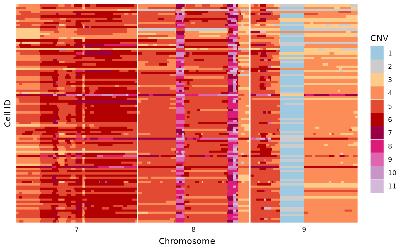
This plot is a simplified alternative to the methods described in the heatmaps vignette. There are no additions, like trees and annotations, but works for a variety of quick inspections.
dlptools::basic_tile_plot(
  # just filtering to make the plot smaller for this demonstration
  dplyr::filter(ex_reads, chr %in% c(7:9))
)
To help with plotting, a variety of commonly use color palettes are available:
# standard state colors
dlptools::CNV_COLOURS
#>         0         1         2         3         4         5         6         7
#> "#3182BD" "#9ECAE1" "#CCCCCC" "#FDCC8A" "#FC8D59" "#E34A33" "#B30000" "#980043"
#>         8         9        10       11+        11
#> "#DD1C77" "#DF65B0" "#C994C7" "#D4B9DA" "#D4B9DA"

# typically used allele specific colors
dlptools::ASCN_COLORS
#>       0|0       1|0       1|1       2|0       2|1       3|0       2|2       3|1
#> "#3182BD" "#9ECAE1" "#CCCCCC" "#666666" "#FDCC8A" "#FEE2BC" "#FC8D59" "#FDC1A4"
#>       4|0         5         6         7         8         9        10        11
#> "#FB590E" "#E34A33" "#B30000" "#980043" "#DD1C77" "#DF65B0" "#C994C7" "#D4B9DA"
#>       11+
#> "#D4B9DA"

# typically used phase colors
dlptools::ASCN_PHASE_COLORS
#>     A-Hom     B-Hom  A-Gained  B-Gained  Balanced
#> "#56941E" "#471871" "#94C773" "#7B52AE" "#d5d5d4"

# typically BAF scale is a circlize::colorRamp2 spanning
# standard green-grey-purple used for ASCN colors
# dlptools::BAF_COLORS
Data Importing
If you’ve followed a semi-standard approach for downloading such as this:
# bash
cd where/to/save/my_dlp/

ticket="SC-8382"
azcopy copy https://singlecellresults.blob.core.windows.net/results/${ticket}/results/annotation/ ${ticket} --recursive
azcopy copy https://singlecellresults.blob.core.windows.net/results/${ticket}/results/hmmcopy/ ${ticket} --recursive
which produces a directory with this sort of structure:
├── SC-8382
│   ├── annotation
│   │   ├── metrics.csv.gz
│   │   ├── #[...other files ...]
│   └── hmmcopy
│   │   ├── #[...other files ...]
│       ├── reads.csv.gz
│       ├── segments.csv.gz
├── SC-8408
│   ├── annotation
│   │   ├── metrics.csv.gz
│   │   ├── #[...other files ...]
│   └── hmmcopy
│   │   ├── #[...other files ...]
│       ├── reads.csv.gz
│       ├── segments.csv.gz
├── SC-8650
then there are some functions that can help with loading data from these into a consistent dataframe:
dlp_dir <- "/where/to/save/my_dlp/"

# loading metrics
metrics <- dlptools::import_dlp_files(dlp_dir, "metrics")

# loading reads
reads_df <- dlptools::import_dlp_files(dlp_dir, "reads")

# loading segments...but generally this isn't a great idea
# segs_df <- dlptools::import_dlp_files(dlp_dir, "segments")
Other
Phylogenetic trees made by Stika take some formatting before they can be plotted:
dlptools::format_sitka_tree()this function drops locus tips and removes the
cell_ part of cell id names on tips. This way, the trees
can be aligned to cell ids in the heatmaps.